Introduction to Time Series Feature Engineering
Understanding Time Series Data
Time series data represents observations measured over successive time intervals. This type of data is prevalent in numerous fields, including finance, economics, and environmental science, where understanding patterns and trends over time is crucial. Analyzing time series data can reveal valuable insights into underlying processes and predict future behavior. Recognizing the temporal dependencies within the data is fundamental to effective analysis.
Key characteristics of time series data include the inherent order of observations and the potential for autocorrelation, where values at one point in time are related to values at other points. Understanding these characteristics is vital for developing appropriate analytical techniques and models.
Key Concepts in Time Series Analysis
Time series analysis involves various concepts, including seasonality, trend, and cyclical patterns. Seasonality refers to repeating patterns in the data over a fixed time period, such as daily, weekly, or yearly fluctuations. Understanding these patterns is essential for removing their influence and isolating other factors.
Trends represent long-term movements in the data. Identifying trends is critical for understanding the overall direction of the time series and for making future predictions. Cyclical patterns represent oscillations or fluctuations in the data that repeat over a longer period. Recognizing these patterns can be crucial for forecasting and making informed decisions.
Methods for Time Series Analysis
Numerous methods exist for analyzing time series data, ranging from simple visual inspection to complex statistical models. Visual methods, such as plotting the data over time, can reveal trends, seasonality, and other patterns. These methods provide a quick overview of the data and can suggest potential modeling approaches.
Statistical modeling techniques, such as autoregressive integrated moving average (ARIMA) models, are powerful tools for forecasting and understanding the dynamics of time series data. These models capture the relationships between observations at different time points and can provide more accurate predictions compared to simple visual inspection. Other approaches like exponential smoothing models are also valuable for handling specific characteristics of time series data.
Applications of Time Series Analysis
Time series analysis has a wide range of applications across various industries. In finance, it's used for forecasting stock prices, predicting market trends, and managing risk. In economics, it's applied to analyze macroeconomic indicators, predict economic growth, and evaluate policy effectiveness.
In environmental science, it's used to model climate change, predict weather patterns, and monitor pollution levels. Furthermore, time series analysis is critical in numerous other fields, including healthcare, engineering, and telecommunications, where understanding patterns over time is vital for making informed decisions and developing effective strategies.
Common Time Series Feature Engineering Techniques
Data Transformation Techniques
Transforming raw time series data into a suitable format for machine learning models is crucial for accurate forecasting and analysis. This often involves techniques like normalization, standardization, and discretization to ensure that features have a consistent scale and distribution. Normalization scales data to a specific range, often 0 to 1, while standardization centers data around zero with a unit variance. Understanding the characteristics of your data is essential in choosing the right transformation.
Discretization, on the other hand, converts continuous data into discrete categories, which can be beneficial for certain algorithms. This approach can help to reduce the complexity of the data and improve the performance of models that are sensitive to the scale of the input features.
Lag Features
Lag features are a fundamental technique in time series analysis, capturing the relationship between past values and current values. By creating lagged variables, we can incorporate historical information into the current prediction. For instance, a lag-1 feature represents the value of the time series from the previous time step, a lag-2 feature represents the value from two time steps ago, and so on. Analyzing these lags can reveal patterns and trends in the data that might not be apparent otherwise.
This method is particularly useful when dealing with time-dependent processes, where current behavior is influenced by past behavior. The selection of the appropriate lag order is critical for optimal model performance and often involves experimentation to find the most informative lag values.
Rolling Statistics
Rolling statistics, such as rolling mean and rolling standard deviation, provide insights into the recent behavior of a time series. These statistics are calculated over a sliding window of data points, offering a dynamic view of the data. This approach is very effective for identifying trends, seasonality, or other patterns that may emerge over time.
By calculating rolling statistics, we can detect periods of high volatility or unusual behavior in the time series. This information can be used to improve the accuracy of forecasts or to identify potential anomalies.
Seasonality Extraction
Seasonality extraction is an essential feature engineering technique for time series data. Seasonality refers to repeating patterns of data fluctuations over specific time intervals, such as daily, weekly, or yearly cycles. Identifying and extracting these patterns is vital for accurate modeling, as ignoring them can lead to inaccurate predictions.
Techniques for extracting seasonality include Fourier transforms and decomposition methods. These methods can effectively separate the seasonal component from the trend and noise components of the time series, allowing for a more accurate analysis of the underlying data patterns.
Feature Scaling
Feature scaling is an important step in time series analysis. It ensures that features with different ranges don't disproportionately influence the model. Common techniques include min-max scaling and standardization (z-score normalization). Min-max scaling scales the features to a specific range, often between 0 and 1. Standardization, on the other hand, centers the data around zero with a unit variance.
Proper scaling is crucial for algorithms that are sensitive to feature magnitudes, such as support vector machines and some neural networks. This step ensures a more balanced and accurate model.
Time-Based Features
Creating time-based features from the original time stamps can be very informative. This involves extracting information from the time component, such as the day of the week, month, or quarter. These features can capture any inherent patterns related to the time of the data.
For instance, sales data might be influenced by the day of the week, with higher sales on weekends. By including these time-based features, we can better capture these patterns and improve the accuracy of our predictions.
Cyclical Features
Identifying cyclical patterns in time series data is important for accurate forecasting. These patterns can represent recurring fluctuations in the data, such as monthly or annual cycles. Techniques like Fourier transforms can help extract these cycles and represent them as features.
Including cyclical features often improves model performance by accounting for the repeating patterns in the data. This leads to more accurate and reliable predictions, especially for time series with recurring fluctuations.
Seasonal Features and Cyclical Patterns
Understanding Seasonal Patterns
Seasonal patterns in time series data are recurring fluctuations that occur at regular intervals, typically tied to calendar cycles like months, quarters, or years. These patterns are crucial to understanding the underlying dynamics of the data and can significantly impact forecasting accuracy. Recognizing and modeling seasonal patterns helps us anticipate future trends and adjust our models accordingly, leading to more reliable predictions. Identifying these cycles often involves examining the data's behavior over multiple years or seasons, looking for consistent peaks and troughs.
A good example of a seasonal pattern is the spike in retail sales around the holidays. This predictable increase in demand allows businesses to plan their inventory management and marketing strategies more effectively. Similarly, agricultural production often displays seasonal patterns, with harvests occurring at specific times of the year. Accounting for these patterns is essential to building accurate models that capture the inherent variability in the data.
Modeling Cyclical Components
Cyclical patterns in time series data represent longer-term, undulating fluctuations that don't adhere to strict calendar cycles. These fluctuations often have a wave-like shape, lasting for several years or even decades. Understanding these cyclical components is vital for accurate forecasting, as they can significantly influence the overall trend of the data. Recognizing and modeling these patterns allows us to anticipate periods of growth and decline, which can be particularly useful in financial markets or economic analysis.
Identifying cyclical patterns requires careful analysis of historical data, often employing techniques like spectral analysis or autocorrelation plots. These techniques can help us isolate the cyclical component from other elements of the data, enabling us to predict future fluctuations more precisely. Accurate modeling of cyclical patterns is essential to account for potential market turning points, allowing businesses to adapt their strategies accordingly.
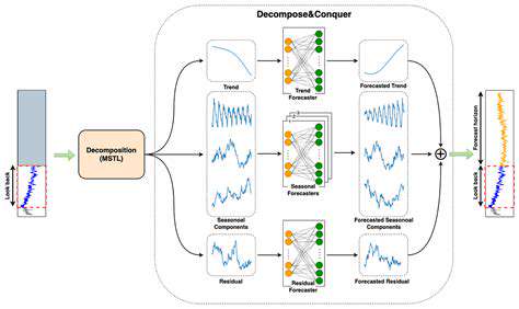
Handling Trend and Seasonality Together
Many time series exhibit both trends and seasonal patterns. Successfully modeling these complex relationships requires techniques that can disentangle these components. A common approach involves decomposing the time series into its constituent parts, allowing us to analyze and model each component individually. This decomposition often involves techniques like the moving average or exponential smoothing, which can help to identify and separate the trend and seasonality from the noise in the data.
The ability to separate these components is essential for accurate forecasting. By understanding the independent contributions of trend and seasonality, we can create more robust models that account for both long-term and short-term fluctuations. This integrated approach leads to more reliable predictions and enables better decision-making in various contexts.
Feature Engineering for Seasonality
Feature engineering plays a crucial role in effectively capturing seasonal patterns. Creating features that represent the seasonal components of the data allows us to feed this information directly into our forecasting models. A common technique involves creating dummy variables for each season or month, enabling the model to learn how each season affects the target variable.
Additionally, creating features that capture the seasonality's magnitude or phase can further enhance the model's ability to anticipate future patterns. These engineered features can lead to a more accurate representation of the cyclical patterns and contribute to more precise forecasts for time series data.
Using Lagged Variables for Cyclicality
Lagged variables are powerful tools for capturing cyclical components in time series data. Introducing lagged versions of the target variable as features allows the model to learn from past values and identify patterns. This approach can be particularly effective in capturing the cyclical nature of the data, as it allows the model to recognize recurring fluctuations over time.
Analyzing the relationship between the current value and past values can reveal cyclical patterns and potentially predict future behavior. The inclusion of these lagged variables often improves the model's ability to forecast cyclical patterns, particularly when combined with other feature engineering techniques.
Decomposition Methods and Their Application
Decomposition methods are valuable techniques for isolating trend, seasonality, and noise components in time series data. These methods, such as the multiplicative or additive decomposition models, can be used to separate the different components, enabling a more detailed analysis of each element. By isolating these components, we can gain a deeper understanding of the factors influencing the data's fluctuations.
Furthermore, decomposition techniques can help in feature engineering by creating new features representing the extracted components. These new features can be used to improve the accuracy and robustness of time series forecasting models by providing more relevant information about the underlying dynamics of the data.
Evaluation Metrics for Seasonal Data
Evaluating the performance of models on time series data with seasonal patterns requires specialized metrics. Standard regression metrics might not adequately capture the nuances of seasonal variations. Metrics like the Mean Absolute Percentage Error (MAPE), Root Mean Squared Error (RMSE), and Mean Absolute Deviation (MAD) are often used to assess forecasting accuracy, but these should be interpreted in the context of seasonal patterns. These metrics provide a measure of how well the model captures the cyclical and trend components of the data.
Comparing models using these metrics helps to identify models that effectively predict future seasonal fluctuations and provide accurate forecasts. Understanding the context of these metrics is critical for drawing meaningful conclusions about the model's performance on seasonal data.